Complexity reduction
Large grids analysed over many time steps can be slow and memory-hungry. eDisGo can reduce both the spatial size (number of buses) and the temporal size (number of time steps) of a problem.
Spatial complexity reduction
In plain terms
Spatial reduction merges nearby buses into a smaller set of representative buses, keeping the electrical behaviour as close as possible to the original grid. This shrinks the grid for faster power flow and optimisation.
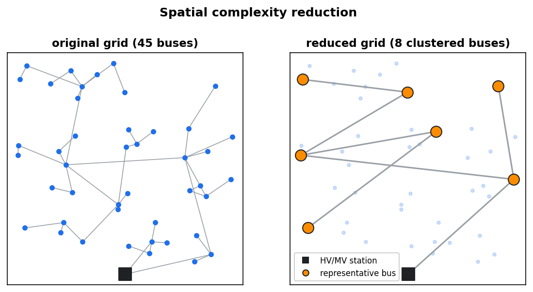
Fig. 11 Spatial complexity reduction clusters buses along the grid into a smaller set of representative buses. Because the clusters are connected parts of the grid, the reduced grid stays radial — each reduced line aggregates real lines.
How it works
Call spatial_complexity_reduction(). The procedure has
two steps: a busmap is built that maps every original bus to a clustered bus, and
the eDisGo object is then reduced according to that busmap (lines are recalculated
and sometimes merged). Parts of the method are based on the spatial clustering of
[PyPSA].
All buses must have coordinates so that line lengths can be derived from the
Euclidean distance and a detour factor. If your grid has no coordinates, set
apply_pseudo_coordinates=True (the default) to compute coordinates from the
radial grid topology.
Parameters:
mode— the clustering method:"kmeans"— assign buses to K-Means cluster centres."kmeansdijkstra"— assign to the nearest cluster centre along the grid graph (Dijkstra distance)."aggregate_to_main_feeder"— assign to the nearest node of the main feeder (the longest path in the feeder)."equidistant_nodes"— place nodes equidistantly along the main feeder.
cluster_area— where clustering is applied:"grid","feeder"or"main_feeder". Note that"aggregate_to_main_feeder"and"equidistant_nodes"only work withcluster_area="main_feeder".reduction_factor— \(n_\text{buses} = k_\text{reduction}\cdot n_\text{buses, cluster area}\); a smaller factor means a stronger reduction.reduction_factor_not_focused— reduce non-critical areas (no voltage or overloading problems in the worst case) more strongly than the focus areas.
For more control you can run the underlying functions directly:
from edisgo.tools.spatial_complexity_reduction import make_busmap, apply_busmap
from edisgo.tools.pseudo_coordinates import make_pseudo_coordinates

edisgo_obj = make_pseudo_coordinates(edisgo_obj)
busmap_df = make_busmap(
    edisgo_obj,
    mode="kmeans",
    cluster_area="feeder",
    reduction_factor=0.25,
)
edisgo_reduced, linemap_df = apply_busmap(edisgo_obj, busmap_df)
See [SCR] and [HoerschBrown] for the theory.
Temporal complexity reduction
The number of analysed time steps can be reduced by keeping only the grid-critical
ones. reinforce() does this when called with
reduced_analysis=True: it picks the most critical steps with
get_most_critical_time_steps()
(ranked by the worst voltage and line-loading issues, by default weighted by the
estimated grid-expansion costs; whole worst-case intervals can be selected with
get_most_critical_time_intervals()).
The flexibility optimisation uses a separate step selection in
edisgo.opf.timeseries_reduction —
get_steps_curtailment() and
get_steps_storage() select and expand the
critical time steps, while
get_linked_steps() then groups them into
representative steps for the OPF.
Memory
reduce_memory() downcasts the stored time-series, results,
heat-pump and overlying-grid DataFrames to smaller dtypes (float32 by default),
lowering memory use without changing the grid.
References
Malte Jahn, Analyse der Auswirkungen räumlicher Komplexitätsreduktion auf
die Verteilnetzausbauplanung mit Flexibilitäten (in German; “Analysis of the
effects of spatial complexity reduction on distribution grid expansion planning
with flexibilities”), master’s thesis, Technische Universität Berlin (in
cooperation with the Reiner Lemoine Institut), 2022.
PDF
The four clustering modes offered by
spatial_complexity_reduction() ("kmeans",
"kmeansdijkstra", "aggregate_to_main_feeder" and "equidistant_nodes")
and the reduction_factor_not_focused option for reducing non-critical areas
more strongly are developed and evaluated there.
Jonas Hörsch, Tom Brown: The role of spatial scale in joint optimisations of generation and transmission for European highly renewable scenarios, arXiv:1705.07617.