Power flow analysis

In plain terms

A power flow computes the voltage at every bus and the current/loading on every line and transformer for a given set of loads and generation. eDisGo uses it to find where the grid is overloaded or where voltages leave the allowed band. It is the measurement step that both reinforcement and the flexibility optimisation build on.

In a typical eDisGo study the power flow is run over a whole future-scenario time series — not a single assumed situation — so you see when and where problems occur across the analysed period.

How it works

analyze() runs a non-linear AC power flow using PyPSA. All loads and generators are modelled as PQ nodes (fixed active and reactive power), and the slack is placed at the secondary side of the HV/MV substation — i.e. the overlying grid is assumed to balance the distribution grid at that point.

The power flow is solved for the time steps in timeindex, or for a subset passed via the timesteps argument. Internally the eDisGo object is converted to a PyPSA network with to_pypsa().

The extent of the power flow is controlled by mode:

• None (default) — the whole grid (MV and all LV grids);

• "mv" — only the MV grid, with the LV grids aggregated at the primary side of their MV/LV stations;

• "mvlv" — like "mv" but the LV grids are aggregated at the station’s secondary side;

• "lv" — a single LV grid (selected via lv_grid_id).

When the power flow does not converge, troubleshooting_mode helps: "lpf" seeds the non-linear power flow with a preceding linear power flow, and "iteration" ramps the loads and generators up from range_start to their full value over range_num steps, re-seeding each step. scale_timeseries applies a uniform scaling factor to the power-flow input, and raise_not_converged (default True) decides whether non-convergence raises an error or is only reported; analyze returns the converging and non-converging time steps.

Which time series?

What the power flow is run over is set beforehand. There are two routes:

• Real future-scenario time series (the main use). Set a real time index with set_timeindex(), then load the scenario’s time series — fluctuating generator and conventional-load profiles from the OpenEnergy DataBase via set_time_series_active_power_predefined(), and the component data (generators, heat pumps, electromobility, …) via the import_* methods — all for a scenario such as "eGon2035". analyze() is then run over the whole period. This is the workflow eDisGo is built for; see Time series and Data sources, and the worked eDisGo full workflow walkthrough.

• Worst-case analysis (a quick alternative). set_time_series_worst_case_analysis() synthesises just two extreme operating points for a fast, conservative planning check, without any scenario data (Worst-case).

Physics

At each bus the complex nodal power balance must hold,

\[S_i = P_i + \mathrm{j}\,Q_i = V_i \sum_k Y_{ik}^* \, V_k^*\]

where \(V_i\) is the complex bus voltage and \(Y\) the nodal admittance matrix built from line and transformer impedances. PyPSA solves this non-linear system with a Newton–Raphson iteration. The results — bus voltages (v_res), apparent powers (s_res) and currents (i_res) — are then compared against the technical limits in Grid reinforcement.

Load case and feed-in case

These are not a way of running the power flow — they are how each operating point is classified so that the correct limits are checked. The two cases describe opposite physical risks, and each is checked against its own limit:

• Load case — high demand, low generation. Power flows from the HV grid into the distribution grid; the risks are overloading from the import and undervoltage — the voltage drops along a feeder. Checked against the allowed voltage drop and the load-case load factors.

• Feed-in case — high generation, low demand. Power flows back to the HV grid (reverse power flow at the HV/MV substation); the risks are reverse overloading and overvoltage — the voltage rises at the generator buses. Checked against the allowed voltage rise and the feed-in-case load factors.

The allowed voltage band is asymmetric — the permitted rise and drop are different numbers — which is exactly why it matters which case applies. For example (defaults in config_grid_expansion), an MV grid may rise by 5 % but only drop by 1.5 %, while an LV grid may rise by 3.5 % but drop by 6.5 %. The load factors are likewise set per case. So “load case / feed-in case” really just answers: which limit do I check this operating point against — the undervoltage one or the overvoltage one?

With real time series every analysed time step is classified for the network as a whole by the sign of the residual load at the HV/MV substation (\(\sum \text{load} - \sum \text{generation} - \sum \text{storage discharge}\)): a non-negative residual (including exactly zero) ⇒ load case, a negative residual ⇒ feed-in case (grid losses are neglected for this classification; see timesteps_load_feedin_case()). The worst-case analysis (Worst-case) instead builds only these two extreme points directly, from simultaneity (scale) factors in config_timeseries.

Note

Do not confuse this with worst-case time series. Load case / feed-in case is a classification that applies to any time series — with real time series every single time step is tagged as one or the other. The worst-case analysis is just the special case where the time series consists of exactly one load-case point and one feed-in-case point; that overlap is why the two are easy to mix up, but they are not the same thing.

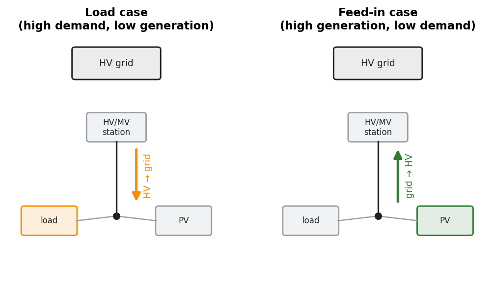
Fig. 1 The two situations, by power-flow direction, that decide which limits apply — not the only thing analysed. With real time series each analysed time step falls into one of them; the worst-case analysis builds only these two extreme points.

For the non-linear optimal power flow used for flexibility scheduling, see Multi-period optimal power flow.