Multi-period optimal power flow

In plain terms

The optimal power flow (OPF) is the engine that schedules all flexibilities at once. Given the grid, the inflexible loads/generation and the flexibility bands (Flexibility & optimisation), it finds operation schedules for electric vehicles, heat pumps, DSM loads and storage that keep voltages and loadings as healthy as possible — so that little or no grid reinforcement is needed — while respecting every component’s bands. It is a multi-period OPF: all time steps are optimised together, because shifting energy in time only makes sense across time.

Note

The model summarised on this page is developed and described in full mathematical detail in the master’s thesis it is based on:

Maike Held, Netzdienlich optimaler Einsatz von Flexibilitäten in radialen Verteilnetzen basierend auf einem AC-Lastflussmodell (in German), master’s thesis, Technische Universität Berlin (in cooperation with the Reiner Lemoine Institut), 2023. PDF

The equation numbers used below (Eq. (3.x)) follow chapter 3 of that thesis, and the Julia source comments use the same numbering. Consult the thesis for the complete derivation, the modelling assumptions and the validation.

How to run it

edisgo.pm_optimize(
    flexible_cps=flexible_cps,            # EV charging points
    flexible_hps=flexible_hps,            # heat pumps with thermal storage
    flexible_loads=flexible_loads,        # DSM loads
    flexible_storage_units=flexible_storage,
    opf_version=2,
    method="soc",
)

pm_optimize() exports the grid and the flexibility bands, runs the optimisation in a Julia subprocess using PowerModels.jl, and writes the resulting operation schedules back into edisgo.timeseries (and the heat / slack results into edisgo.results). The Julia/Gurobi prerequisites are described in Additional requirements for the optimal power flow.

The four flexibility arrays select which components may be optimised; any component not listed keeps its given time series. Non-flexible storage units operate to optimise self-consumption rather than being scheduled by the OPF.

The grid model: radial branch flow

eDisGo’s OPF uses a radial branch flow model (BFM) — the natural formulation for the tree-shaped distribution grids ding0 produces.

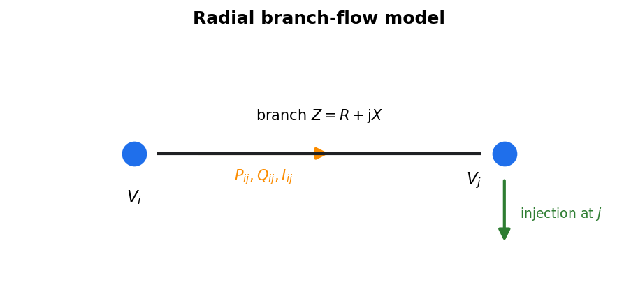
../../_images/branch_flow_model.png — Fig. 6 Radial branch-flow model: for each branch \(i \to j\) the model couples the sending-end power \((P_{ij}, Q_{ij})\), the branch current \(I_{ij}\) and the bus voltages \(V_i, V_j\), with a power balance at every bus.

For every branch and bus the model enforces:

Power balance at each bus — injected active and reactive power equals what flows out on the branches plus losses.
Branch flow / thermal limit — apparent power on a branch stays within its rating, \(S = \sqrt{P^2 + Q^2} \le S_\text{lim}\).
Voltage limits — \(V_\text{min} \le V \le V_\text{max}\) at every bus.
Flexibility constraints — each flexibility’s power and energy bands (Flexibility & optimisation), e.g. for a store the state of energy must stay within \([E_\text{min}, E_\text{max}]\) and the charging requirement must be met by departure.

The coupling between branch power, current and voltage is the quadratic equality

\[P^2 + Q^2 = V^2 \cdot I^2 ,\]

which is what makes an exact AC-OPF non-convex.

All quantities are scaled to per-unit on a common base power s_base (an argument of pm_optimize(), default 1 MVA), which keeps the optimisation numerically well-conditioned.

Solution method: SOC vs. non-convex

The method argument chooses how that quadratic constraint is handled:

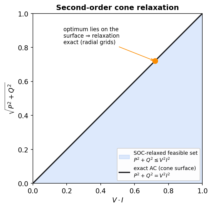
../../_images/soc_relaxation.png — Fig. 7 The SOC relaxation replaces the non-convex equality \(P^2+Q^2=V^2 I^2\) (the cone surface) with the convex inequality \(P^2+Q^2 \le V^2 I^2\) (the filled cone). For radial grids the optimum lies on the surface, so the relaxation is usually *exact*.

"soc" (default) — a second-order cone relaxation replaces the equality \(P^2+Q^2=V^2 I^2\) with the convex inequality \(P^2+Q^2 \le V^2 I^2\). The resulting convex problem is solved with Gurobi and is fast and reliable. For radial grids the relaxation is usually exact (the inequality is tight at the optimum), so the solution is also feasible for the original AC problem; where it is not, the violations are written to a JSON file in opf/opf_solutions/.
"nc" — the non-convex problem with the exact equality, solved with the Ipopt interior-point solver. More accurate in principle but slower and not guaranteed to find the global optimum.
warm_start=True (with method="soc") — additionally runs the non-convex Ipopt OPF, warm-started from the Gurobi SOC solution, to polish the result. Note that this only runs when the SOC solution is already tight; if it is not, the warm start is skipped.

Optimisation versions

The opf_version argument selects the objective and which constraints are active. All versions minimise line losses; they differ in how grid limits and the overlying (high-voltage) grid are treated:

Version	Constraints	Objective
1 (default)	Grid restrictions lifted	minimise line losses and maximum line loading
2	Standard grid restrictions	minimise line losses and grid-related slacks
3	HV requirements added; grid restrictions lifted	minimise line losses, maximum line loading and HV slacks
4	HV requirements added; standard grid restrictions	minimise line losses, HV slacks and grid-related slacks

“Lifting” the grid restrictions (versions 1 and 3) turns hard voltage/loading limits into a penalised objective term (maximum loading), which is useful for assessing how much flexibility could help before deciding on reinforcement. Versions 2 and 4 keep the limits as constraints and penalise the remaining unavoidable violations via slack variables. Versions 3 and 4 additionally honour requirements handed down from the overlying grid (Overlying-grid requirements); if no overlying-grid data is present, they silently fall back to version 2.

The optimisation model in detail

This section describes the actual mathematical program eDisGo assembles and hands to the solver — its decision variables, objective and constraints. It follows the formulation of Held (2023) (see the note at the top of this page), whose chapter-3 equation numbers (Eq. (3.x)) are reused in the Julia source comments; the thesis holds the full derivation. Each block below maps to functions in the Julia OPF API (the variable_*, constraint_* and objective_* families).

Decision variables

At every optimised time step the solver chooses:

the branch-flow state — the active and reactive branch flows \(P_{ij}, Q_{ij}\), the squared branch current \(I_{ij}^2\) and the squared bus voltages \(V_i^2\);
the substation exchange \(P_\text{s}, Q_\text{s}\) with the overlying grid at the slack bus;
one operation variable per flexibility — battery power \(p^\text{bat}\), EV charging power \(p^\text{ev}\), heat-pump electrical power \(p^\text{hp}\) and DSM shift power \(p^\text{dsm}\) — together with the stored-energy state of each store (battery \(e^\text{bat}\), EV \(e^\text{ev}\), thermal store \(e^\text{th}\), DSM \(e^\text{dsm}\));
depending on the version, slack variables that absorb otherwise-infeasible situations (generation curtailment, load shedding, EV and heat-pump shedding, heat-pump operation slacks, overlying-grid slacks) and the auxiliary maximum-line-loading variable.

Objective

All versions minimise the ohmic line losses \(\sum_{ij} I_{ij}^2\, r_{ij}\), summed over all branches and time steps. This term has a double purpose: besides being a sensible grid-friendliness goal, it pushes the squared current \(I_{ij}^2\) downwards onto the boundary of the SOC relaxation, which keeps that relaxation tight — i.e. its solution stays feasible for the original AC problem. Depending on opf_version it is combined with the maximum line loading (versions 1 and 3) and/or weighted penalties on the slack variables (versions 2 and 4) and the overlying-grid requirement slacks (versions 3 and 4). The exact combination is the one listed under Optimisation versions above, implemented by the objective_* functions.

Network constraints (per time step)

Power balance (Kirchhoff’s current law) at every bus — the power arriving on incoming branches equals the power leaving on outgoing branches plus the ohmic losses, plus the net injection of the generators, loads and flexibilities connected to the bus (Eq. (3.3)/(3.4)). Reactive injections of the flexibilities follow from their active power via the power factor.
Voltage-drop equation along every branch, relating the squared voltages at its two ends to the flows, the squared current and the branch impedance (Eq. (3.5)); the slack-bus voltage is fixed to \(1\,\text{p.u.}\)
Current–power–voltage coupling \(P^2 + Q^2 = V^2 I^2\) — kept as the exact non-convex equality (method="nc") or relaxed to the convex inequality \(\le\) (method="soc"); see Solution method: SOC vs. non-convex above (Eq. (3.6)).
Voltage limits \(V_\text{min}^2 \le V_i^2 \le V_\text{max}^2\) (Eq. (3.8)) and thermal / loading limits — a current limit on every branch (versions 2 and 4, Eq. (3.7)) or, when the grid restrictions are lifted (versions 1 and 3), the maximum-line-loading bound that the objective then minimises (Eq. (3.40)).

Flexibility dynamics (across time steps)

The flexibilities are what couple the time steps: a store’s energy at one step depends on the previous step and the power chosen in between. With time-step length \(\Delta t\) and, where applicable, efficiency \(\eta\):

Battery / home storage — the state of energy evolves as \(e^\text{bat}_t = e^\text{bat}_{t-1} - \Delta t\, p^\text{bat}_t\), starting from the given initial charge and returning to a required end value (Eq. (3.9)/(3.10)), and stays within \([E_\text{min}, E_\text{max}]\). eDisGo uses a resistance-based battery model (Stai et al.): each battery is an ideal store at a virtual bus connected to its real bus through a purely resistive virtual line, so that its power-dependent charging/discharging losses appear as ohmic losses on that line — this is the “storage branch” that shows up in the branch-flow results.
Electric vehicles — the charged energy accumulates as \(e^\text{ev}_t = e^\text{ev}_{t-1} + \Delta t\,\eta\, p^\text{ev}_t\) (Eq. (3.25)/(3.26)); it is pinned to the middle of the energy band at the start and end of the horizon, which encodes the charging requirement — the battery must be charged by departure.
Heat pumps with thermal storage — the electrical power, through the coefficient of performance \(\mathrm{COP}\), must cover the building’s heat demand plus the net (dis)charge of the thermal store (\(\mathrm{COP}\cdot p^\text{hp}_t = \dot q^\text{demand}_t + \text{(net thermal-store charge)}\), Eq. (3.19)); the thermal store has its own energy balance with standing losses (Eq. (3.22)/(3.23)).
Demand-side management — the shifted energy \(e^\text{dsm}_t = e^\text{dsm}_{t-1} + \Delta t\, p^\text{dsm}_t\) (Eq. (3.32)/(3.33)) stays within the DSM band and must return to zero by the end of the horizon: shifted load is recovered, not dropped.
Overlying-grid requirements (versions 3 and 4) — the summed dispatch of the addressed flexibility must meet the active power requested by the higher voltage level, up to a penalised slack (Overlying-grid requirements).

Multi-period structure

Each time step is built as one PowerModels network, and the dynamics above link the battery, EV, heat and DSM states across consecutive networks (the Julia build_mn_opf_bf_flex assembles this multi-network problem). This is exactly why the OPF must be solved as one joint multi-period optimisation rather than time step by time step — and why its size grows with the number of time steps, which Complexity reduction helps to contain.

Results and slacks

Operation schedules are written into edisgo.timeseries (charging-point, heat-pump, DSM and storage active power) and can then feed a final reinforce(). Heat-storage states, the slack generator and the optimisation slack variables are written back as well; which slacks exist depends on opf_version (see edisgo.io.powermodels_io.from_powermodels()). Solver and Julia output can be silenced with silence_moi=True.

Note

pm_optimize also declares save_heat_storage, save_slack_gen and save_slacks parameters, but these are currently not forwarded to the conversion and therefore have no effect.

Beyond the schedules, the full raw optimisation result is collected in edisgo.opf_results, an OPFResults object. It holds the solver status and solve time, the per-line branch-flow variables (LineVariables), the heat- and battery-storage trajectories (HeatStorage, BatteryStorage), the exchange with the overlying grid, and the grid slack variables — curtailment and load shedding — (GridSlacks). See its API reference for the full field list.

Performance

Because all time steps are optimised jointly, the problem grows with both grid size and the number of time steps. Use Complexity reduction (spatial reduction and the temporal selection in edisgo.opf.timeseries_reduction) and a per-unit base s_base to keep the problem tractable.